Chapter 5 MLWIC2: Machine Learning for Wildlife Image Classification
MLWIC2 is an R package that allows you either to use trained models for identifying species from North America (using the “species_model”) or to identify if an image is empty or if it contains an animal (using the “empty_animal” model) (Tabak et al. 2020). The model was trained using images from 10 states across the United States but was also tested in out-of sample data sets obtaining a 91% accuracy for species from Canada and 91% - 94% for classifying empty images on samples from different continents (Tabak et al. 2020).
Documentation for using MLWIC2 and the list of species that the model identifies can be found in the GitHub repository https://github.com/mikeyEcology/MLWIC2. In this chapter we illustrate the use of the package and data preparation for model training.
5.1 Set-up
First, you will need to install R software, Anaconda Navigator (https://docs.anaconda.com/anaconda/navigator/), Python (3.5, 3.6 or 3.7) and Rtools (only for Windows computers). Then you will have to install TensorFlow 1.14 and find the path location of Python on your computer. You can find more installation details in the GitHub repository (https://github.com/mikeyEcology/MLWIC2), as well as an example with installation steps for Windows users (https://github.com/mikeyEcology/MLWIC_examples/blob/master/MLWIC_Windows_Set_up.md).
Make sure to install the required versions listed above. Mac users can use the Terminal Application to install Python and TensorFlow. You can use the conda package (https://docs.conda.io/en/latest/) to create an environment that can host a specific version of Python and keep it separated from other packages or dependencies. In the Terminal type:
conda create -n ecology python=3.5
conda activate ecology
conda install -c conda-forge tensorflow=1.14
Once you complete the installation of Python and TensorFlow, use the command-line utility to find the location of Python. Windows users should type: where python. Mac users should type conda activate ecology and then which python.
The output Python location will look something like this: /Users/julianavelez/opt/anaconda3/envs/ecology/bin/python
In R, install the devtools package and MLWIC2 packages. Then, setup your environment using the setup function (Tabak et al. 2020) as shown below, making sure to change the python_loc argument to point to the output path provided in the previous step. You will only need to specify this setup once.
# Uncomment and only run this code once
# if (!require('devtools')) install.packages('devtools')
# devtools::install_github("mikeyEcology/MLWIC2")
# MLWIC2::setup(python_loc = "/Users/julianavelez/opt/anaconda3/envs/ecology/bin/")
Next, download MLWIC2 helper files from here: https://drive.google.com/file/d/1VkIBdA-oIsQ_Y83y0OWL6Afw6S9AQAbh/view. Note, this folder is not included in the repository because of its large size. You must download it and store it in the data/mlwic2 directory.
5.2 Upload/format data
Once the package is installed and the python location is setup, you can run a MLWIC2 model to obtain computer vision predictions of the species present in your images. To run MLWIC2 models, you should use the classify function (see Section 5.3), which requires arguments specifying the path (i.e., location on your computer) for the following three inputs:
- The images that will be classified.
- The filenames of your images.
- The location of the MLWIC2 helper files that contain the model information.
To create the filenames (input 2 above), you will need to create an input file using the make_input function (Tabak et al. 2020). This will create a CSV file with two columns, one with the filenames and the other one with a list of class_ID’s required to use MLWIC2 for classifying images or training a model. When using the make_input function to create the CSV file, you can select different options depending whether or not you already have filenames and images classified (type ?make_input in R for more options).
We will use option = 4 to find filenames associated with each photo using MLWIC2 and recursive = TRUE to specify that photos are in subfolders organized by camera location. We then read the output using the read_csv function (Wickham 2017). Let’s first load required libraries for reading data and to use MLWIC2 functions.
library(tidyverse) # for data wrangling and visualization, includes dplyr
library(MLWIC2)
library(here) # to allow the use of relative paths while reading data
When using the make_input function with your data, you must provide the paths indicating the location of your images (path_prefix) and the output directory where you want to store the output. The make_input function will output a file named image_labels.csv which we renamed as images_names_classify.csv and included it with the files associated with this repository. We provide a full illustration of the use of make_input and classify in Section 5.6 using a small image set included in the repository.
# The code below won't be executed. For using it you must replace:
# - the "path_prefix" with the path to the directory holding your images
# - the "output_directory" with the directory where you want to store the output
#   from running MLWIC2
make_input(path_prefix = "/Volumes/ct-data/CH1/jan2020",
           recursive = TRUE,
           option = 4,
           find_file_names = TRUE,
           output_dir = here("data", "mlwic2"))

file.rename(from = "data/mlwic2/image_labels.csv", to = "data/mlwic2/images_names_classify.csv")
We then read in this file containing the image filenames and look at the first few records. We will use the here package (Müller 2017) to tell R that our file lives in the ./data/mlwic2 directory and specify the name of our file images_names_classify.csv.
# inspect output from the make_input function
image_labels <- read_csv(here("data","mlwic2","images_names_classify.csv"))
head(image_labels)
## # A tibble: 6 × 2
## `A01/01080001.JPG` `0`
## <chr> <dbl>
## 1 A01/01080002.JPG 0
## 2 A01/01080003.JPG 0
## 3 A01/01080004.JPG 0
## 4 A01/01080005.JPG 0
## 5 A01/01080006.JPG 0
## 6 A01/01080007.JPG 05.3 Process images - AI module
Once you have the CSV file with image filenames (images_names_classify.csv), you can proceed to run the MLWIC2 models. It is possible to use parallel computing to run the models more efficiently. This will require specifying a number of cores that you want to use while running the models. To do that, first you need to know how many cores (i.e., processors in your computer) are available, which you can determine using the detectCores function in the parallel package (R Core Team 2021).
## [1] 4If you have 4 cores, then you can use 3 cores for running the MLWIC2 model using the classify function (Tabak et al. 2020) and the num_cores argument. This assures that you leave one core for your computer to perform other tasks.
Other arguments for the classify function include:
path_prefix: absolute path of the location of your camera trap photos.data_info: absolute path of theimages_names_classify.csvfile (i.e., the output from themake_inputfunction).
model_dir: absolute path of MLWIC2 helper files folder.python_loc: absolute path of Python on your computer.os: specification of your operating system (here “Mac”).make_output: use TRUE for a ready-to-read CSV output.
To complete this step, you would need to change the file paths to indicate where the files are located on your computer. Note that this step took approximately 5 hours to process 110,457 photos (run on a macOS Mojave with a 2.5 GHz Intel Core i5 Processor and 8GB 1600 MHz DDR3 of RAM).
classify(path_prefix = "/Volumes/ct-data/CH1/jan2020/",
         data_info = here("data", "mlwic2", "images_names_classify.csv"),
         model_dir = here("data", "mlwic2", "MLWIC2_helper_files/"),
         python_loc = "/Users/julianavelez/opt/anaconda3/envs/ecology/bin/", # absolute path of Python on your computer
         os = "Mac", # specify your operating system; "Windows" or "Mac"
         make_output = TRUE,
         num_cores = 3
         )
5.4 Assessing AI performance
As with other AI platforms, it is recommended to evaluate model performance with your particular data set before using an AI model to classify all your images. This involves classifying a subset of your photos and comparing those classifications with predictions provided by MLWIC2 (i.e., we will compare human vs. computer vision). Let’s start by formatting the human vision data set.
5.4.1 Format human vision data set
To read the file containing the human vision classifications for a subset of images, we tell R the path (i.e., directory name) that holds our file. Again, we use the here package (Müller 2017) to tell R that our file lives in the ./data/mlwic2 directory and specify the name of our file images_hv_jan2020.csv. We then read our file using the read_csv function (Wickham 2017).
The human vision data set (images_hv_jan2020.csv) was previously cleaned to remove duplicated records and to summarize multiple rows that reference animals of the same species identified in the same image (see Chapter 3) for details about these steps).
MLWIC2 provides predictions for species from North America (see list of predicted species here https://github.com/mikeyEcology/MLWIC2/blob/master/speciesID.csv). However, you can also use the MLWIC2 empty_animal model for distinguishing blanks from images containing an animal. For our example with species from South America, we will use the species_model as we want to evaluate model performance for predicting species present both in North and South America (e.g., white-tailed deer and puma).
We created two CSV files containing the taxonomy for species in computer and human vision. These taxonomy files have the same format for species name (scientific notation stored in the species column). We join the taxonomy files to our records to be able to evaluate model performance based on common scientific notation. We join the taxonomy to each visions using the common_name column.
tax_ori <- read_csv(here("data", "mlwic2", "tax_hv_ori.csv"))

hv_tax <- human_vision %>% left_join(tax_ori, by = "common_name")
As the “Blank” category is represented as “NA” in the species column, we make sure it is correctly labeled in that column.
5.4.2 Format computer vision data set
Let’s read the MLWIC2 output and the taxonomy file, and remove unwanted patterns in the filenames using str_remove and gsub.
MLWIC2 outputs columns with filename and the top-5 predictions along with their associated confidence values. Filenames are represented as camera_location/image_filename. Note that we have moved the model output to the data/mlwic2 folder from its original location (in the same folder as the MLWIC2_helper_files that you previously downloaded). We join the taxonomy file to MLWIC2 output, remove the “Vehicle” and the “Human” records, and assign the “Blank” label in the species column for empty images.
mlwic2 <- read_csv(here("data", "mlwic2", "MLWIC2_output_ori.csv"))

tax_mlwic2 <- read_csv(here("data", "mlwic2", "tax_mlwic2.csv"))

mlwic2 <- mlwic2 %>%
        select(fileName, guess1, confidence1) %>%
        rename(common_name = guess1,
               filename = fileName,
               confidence_cv = confidence1) %>%
        mutate(filename = str_remove(filename, pattern = "'")) %>%
  mutate(filename = str_remove(filename, "b/Volumes/ct-data/CH1/jan2020/"),
         filename = str_remove(filename, pattern = "'")) %>%
  mutate(filename = gsub(x=filename, pattern ="[0-9]*EK113/", replacement = ""))

mlwic2_tax <- mlwic2 %>% left_join(tax_mlwic2, by = "common_name")

mlwic2_tax <- mlwic2_tax %>%
  filter(!common_name %in% 25 & !common_name %in% 11) %>%
  mutate(species = case_when(common_name == 27 ~ 'Blank', TRUE ~ species))
We check if there are multiple predictions for the same filename in computer vision (see Chapter 3 for details about performing this step with human vision). For a filename with multiple predictions of the same species, we only keep the record with the highest confidence value using the top_n function. We also create a sp_num column, which can then be used to identify records with more than one species in an image sp_num > 1.
cv_seq <- mlwic2_tax %>%
        group_by(filename, species) %>%
        top_n(1, confidence_cv) %>% # keep highest value of same class
        group_by(filename, species) %>%
        distinct(filename, species, confidence_cv, .keep_all = TRUE) # for filenames with the same confidence value, keep a single record


cv <- cv_seq %>%
        group_by(filename) %>%
        mutate(sp_num = length(unique(common_name))) %>%
        group_by(filename) %>%
        filter(!(common_name == "Blank" & sp_num > 1)) %>% # for groups with num_classes > 1, remove blanks
        mutate(sp_num = length(unique(common_name))) # re-estimate sp_num with no blanks
5.4.3 Merging computer and human vision data sets
We can use various “joins” (Wickham et al. 2019) to merge computer and human vision together so that we can evaluate the accuracy of MLWIC2. First, however, we will eliminate any images that were not processed by both humans and AI.
# Determine which images have been viewed by both methods
ind1 <- cv$filename %in% hv$filename # in both
ind2 <- hv$filename %in% cv$filename # in both

cv <- cv[ind1,] # eliminate images not processed by hv
hv <- hv[ind2,] # eliminate images not processed by cv

# Number of photos eliminated
sum(ind1 != TRUE) # in cv but not in hv
## [1] 4690## [1] 4612Now, we can use:
- an
inner_joinwithfilenameandspeciesto determine images that have correct predictions (i.e., images with the same class assigned by computer and human vision) - an
anti_joinwithfilenameandspeciesto determine which records in the human vision data set have incorrect predictions from computer vision. - an
anti_joinwithfilenameandspeciesto determine which records in the computer vision data set have incorrect predictions.
We assume the classifications from human vision to be correct and distinguish them from MLWIC2 predictions. The MLWIC2 predictions will be correct if they match a class assigned by human vision for a particular record and incorrect if the classes assigned by the two visions differ.
hv <- hv %>% select(filename, species)
cv <- cv %>% select(filename, species, confidence_cv)

# correct predictions

matched <- cv %>% inner_join(hv,
                by = c("filename", "species"),
                suffix = c("_cv", "_hv")) %>%
        mutate(class_hv = species) %>%
        mutate(class_cv = species)

# incorrect predictions in hv set
hv_only <- hv %>% anti_join(cv,
                by = c("filename", "species"),
                suffix = c("_hv", "_cv")) %>%
        rename(class_hv = species)

# incorrect predictions in cv set
cv_only<- cv %>% anti_join(hv,
               by = c("filename", "species"),
               suffix = c("_cv", "_hv")) %>%
        rename(class_cv = species)
We then use left_join to merge the predictions from the cv_only (computer vision) data set onto the records from the hv_only (human vision) data set.
We combine the matched and mismatched data sets. Then, we set a 0.65 confidence threshold to assign MLWIC2 predictions and evaluate model performance. “NA” values in the species column correspond to categories representing higher taxonomic levels with no species classification available.
both_visions <- rbind(matched, hv_mismatch)

both_visions <- both_visions %>%
  mutate(class_hv = case_when(is.na(class_hv) ~ "Higher tax level", TRUE ~ class_hv)) %>%
  mutate(class_cv = case_when(is.na(class_cv) ~ "Higher tax level", TRUE ~ class_cv))

both_visions_65 <- both_visions
both_visions_65$class_cv[both_visions_65$confidence_cv < 0.65] <- "No CV Result"
5.4.4 Confusion matrix and performance measures
Using the both_visions_65 data frame, we can estimate a confusion matrix using the confusionMatrix function from the caret package (Kuhn 2021). The confusionMatrix function requires a data argument of a table with predicted and observed classes, both as factors and with the same levels. We use the factor function (R Core Team 2021) to convert class names into factor classes. We specify mode = "prec_recall" when calling the confusionMatrix function (Kuhn 2021) to estimate the precision and recall for the MLWIC2 classifications.
library(caret) # to inspect model performance
library(ggplot2) # to plot results

all_class <- union(both_visions_65$class_cv, both_visions_65$class_hv)
cm_mlwic2 <- table(factor(both_visions_65$class_cv, all_class),
               factor(both_visions_65$class_hv, all_class)) # table(pred, truth)
cm_mlwic2 <- confusionMatrix(cm_mlwic2, mode="prec_recall")
We then group the data by class_cv andclass_hv and count the number of observations using n() inside summarise. Then, we filter classes with at least 20 records and use the intersect function to get the pool of classes shared in the output of computer and human vision. Finally, we keep records containing classifications at the species level, but the confusion matrix and model performance metrics can also be estimated for higher taxonomic levels.
class_num_cv <- both_visions %>% group_by(class_cv) %>%
  summarise(n = n()) %>%
  filter(n >= 20) %>%
  pull("class_cv") %>%
  unique()
class_num_hv <- both_visions %>% group_by(class_hv) %>%
  summarise(n = n()) %>%
  filter(n >= 20) %>%
  pull("class_hv") %>%
  unique()

(class_num <- intersect(class_num_cv, class_num_hv))
## [1] "Blank" "Higher tax level" "Odocoileus virginianus"
## [4] "Puma concolor"White-tailed deer and puma are the species shared in the output of computer and human vision, and with at least 20 records in each data set.
Now we can use the confusion matrix to estimate model performance metrics including accuracy, precision, recall and F1 score (See Chapter 1 for metrics description).
## [1] 0.03classes_metrics <- cm_mlwic2 %>%
pluck("byClass") %>%
as.data.frame() %>%
select(Precision, Recall, F1) %>%
rownames_to_column() %>%
rename(species = rowname) %>%
mutate(species = str_remove(species, pattern = "Class: ")) %>%
filter(species %in% sp_num) %>%
mutate(across(is.numeric, ~round(., 2)))5.4.5 Confidence thresholds
Finally, we define a function that allows us to inspect how precision and recall change when different confidence thresholds are used for assigning a prediction made by computer vision. Our function will assign a “No CV Result” label whenever the confidence for a computer vision prediction is below a user-specified confidence threshold. Higher thresholds should reduce the number of false positives but at the expense of more false negatives. We then estimate the same performance metrics for the specified confidence threshold. By repeating this process for several different thresholds, users can evaluate how precision and recall for each species change with the confidence threshold and identify a threshold that balances precision and recall for the different species.
threshold_for_metrics <- function(conf_threshold = 0.7) {
  df <- both_visions
  df$class_cv[df$confidence_cv < conf_threshold] <- "No CV Result"

  all_class <- union(df$class_cv, df$class_hv)
  newtable <- table(factor(df$class_cv, all_class), factor(df$class_hv, all_class)) # table(pred, truth)
  cm <- confusionMatrix(newtable, mode="prec_recall")

  # metrics
  classes_metrics <- cm %>% # get confusion matrix
    pluck("byClass") %>% # get metrics by class
    as.data.frame() %>%
    select(Precision, Recall, F1) %>%
    rownames_to_column() %>%
    rename(class = rowname) %>%
    mutate(conf_threshold = conf_threshold)
  classes_metrics$class <- str_remove(string = classes_metrics$class,
                                      pattern = "Class: ")

  return(classes_metrics) # return a data frame with metrics for every class
}
Let’s look at the distribution of confidence values associated with each species using the geom_bar function (Wickham et al. 2018).
# Plot confidence values
both_visions %>%
  filter(class_cv %in% sp_num & class_hv %in% sp_num)  %>%
  ggplot(aes(confidence_cv, group = class_cv, colour = class_cv)) +
  geom_bar() +
  facet_wrap(~class_cv, scales = "free") +
  labs(y = "Empirical distribution", x = "Confidence values")+
  theme(legend.position="bottom") +
  scale_color_viridis_d()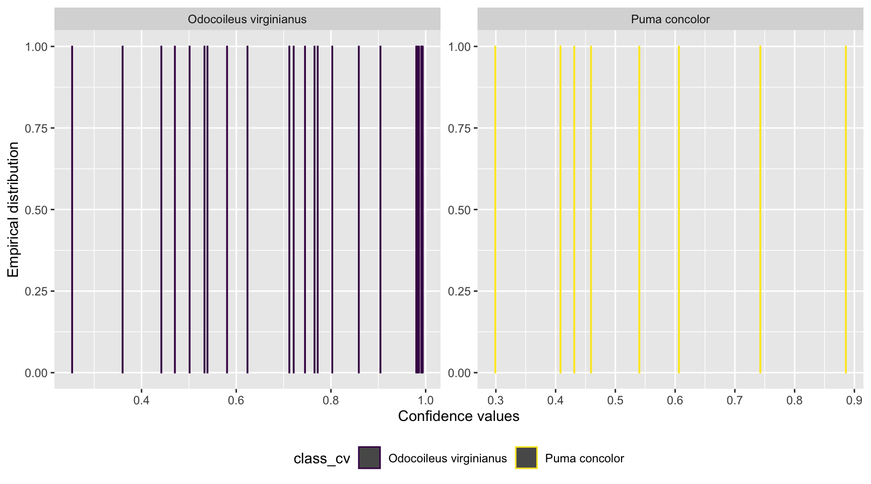
Figure 5.1: Distribution of confidence values associated with species shared by computer and human vision, and with at least 20 records in each data set.
We can see a uniform distribution for both species with records distributed along the full range of confidence values.
Let’s estimate model performance metrics for confidence values ranging from 0.1 to 0.99 using the map_df function (Henry and Wickham 2020) . The map_df function (Henry and Wickham 2020) returns a data frame object. Once we get a data frame of model performance metrics for a range of confidence values, we can plot the results using the ggplot2 package (Wickham et al. 2018).
conf_vector = seq(0.1, 0.99, length=100)
metrics_all_confs <- map_df(conf_vector, threshold_for_metrics)
# Plot Precision and Recall
prec_rec_mlwic2 <- metrics_all_confs %>%
mutate_if(is.numeric, round, digits = 2) %>%
filter(class %in% sp_num) %>%
rename(Species = class, `Confidence threshold` = conf_threshold) %>%
ggplot(aes(x = Recall, y = Precision, group = Species, colour = Species)) +
geom_point(aes(size = `Confidence threshold`)) +
scale_size(range = c(0.01,3)) +
geom_line() +
scale_color_viridis_d() +
xlim(0, 1) + ylim(0, 1)
prec_rec_mlwic2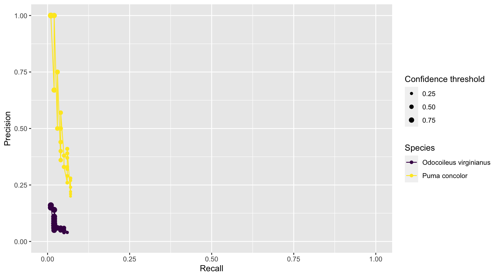
Figure 3.11: Precision and recall for different confidence thresholds for species shared by computer and human vision, and with at least 20 records in each data set. Point sizes represent the confidence thresholds used to accept AI predictions.
We see that as we increase the confidence threshold, precision usually increases and recall decreases (Figure 3.11). Ideally, we would like AI to have high precision and recall, though the latter is likely to be more important in most cases. Remember that precision tells us the probability that the species is truly present when AI identifies the species as being present in an image (Chapter 1). If AI suffers from low precision, then we may have to manually review photos that AI tags as having species present in order to remove false positives. Recall, on the other hand, tells us how likely AI is to find a species in the image when it is truly present. If AI suffers from low recall, then it will miss many photos containing images of species that are truly present. To remedy this problem, we would need to review images where AI says the species is absent in order to reduce false negatives. Predictions from MLWIC2 present low recall for both species likely due to strong differences between the training and test data sets. However, MLWIC2 contains a training module where users can input manually classified images to train a new model and increase accuracy.
5.5 Model training
For training a model, we also need to provide a CSV file containing image filenames. For illustration, we will get the filenames from a small set of images included in the repository (images/train folder), but you will want to train a model with at least 1,000 labeled images per species (Schneider et al. 2020). To get the filenames for those images we can use the make_input function (See Section 5.2); in the argument path_prefix you should provide the path of the directory containing the images. The make_input function will create the image_labels.csv file in the directory provided in the output_dir argument. We rename this file as images_names_train_temp.csv.
# create CSV file with filenames
make_input(path_prefix = here("data","mlwic2","images", "train"),
           option = 4,
           find_file_names = TRUE,
           output_dir = here("data", "mlwic2", "training"))

file.rename(from = "data/mlwic2/training/image_labels.csv",
            to = "data/mlwic2/training/images_names_train_temp.csv")
Once we have the filenames for the training set, we add the corresponding human vision labels for each image using a left_join. Additionally, we recode our species names with numbers as required by the MLWIC2 package and save them as images_names_train.csv; these numbers must be consecutive and should start with 0 (Tabak et al. 2020).
img_labs <- read_csv(here("data", "mlwic2", "training", "images_names_train_temp.csv"),
                     col_names = c("filename", "class"))

hv_train <- read_csv(here("data", "mlwic2", "training", "images_hv.csv"))

imgs_train <- img_labs %>%
  left_join(hv_train, by = "filename") %>%
  select(filename, common_name) %>%
  drop_na(common_name)

names_nums <-  data.frame(common_name = unique(imgs_train$common_name),
                          class_ID = seq(from = 0, to = 9))

imgs_train <- imgs_train %>%
  left_join(names_nums, by = "common_name") %>%
  ungroup() %>%
  select(filename, class_ID)

write_csv(imgs_train, file = "data/mlwic2/training/images_names_train.csv", col_names = FALSE)
We then use the train function to train a new model, where we need to specify arguments that were also used with the classify function (see Section 5.3); these include the path_prefix, model_dir, python_loc, os and num_cores. In the data_info argument we pass the images_names_train.csv file. We also need to specify the number of classes that we want to train the model to predict (e.g., these classes might differ from the 58 classes predicted when using MLWIC2’s built-in AI species model).
We can use retrain = FALSE to train a model from scratch or retrain = TRUE if we want to retrain a pre-specified model using transfer learning.1 For more references on model training see https://github.com/mikeyEcology/MLWIC2.
We specify 55 number of epochs (i.e., the number of times the learning algorithm will iterate on the training data set) (Tabak et al. 2020). Lastly, we specify the directory where we want to store the model using the log_dir_train argument; we use “SA” for “South America”.
train(path_prefix = here("data","mlwic2", "images", "train"),
         data_info = here("data", "mlwic2", "training", "images_names_train.csv"), # absolute path to the make_input output
         model_dir = here("data","mlwic2", "MLWIC2_helper_files/"),
         python_loc = "/Users/julianavelez/opt/anaconda3/envs/ecology/bin/", # absolute path of Python on your computer
         os = "Mac", # specify your operating system; "Windows" or "Mac"
         num_cores = 3,
      num_classes = 22, # number of classes in your data set
      retrain = FALSE,
      num_epochs = 55,
      log_dir_train ="SA"
      )
5.6 Classify using a trained model
Finally you can run the model that you trained using a test image set. You should also get filenames for these images (renamed as images_names_test.csv) and pass it when running the model with the classify function. Model output will contain top-5 predictions for each image with their associated confidence values. Once you have this output, you can verify model performance as described along Section 5.4.
make_input(path_prefix = here("data", "mlwic2", "images", "test"),
           option = 4,
           find_file_names = TRUE,
           output_dir = here("data","mlwic2","training"))
## Your file is located at '/Users/julianavelez/Documents/GitHub/Processing-Camera-Trap-Data-using-AI/data/mlwic2/training/image_labels.csv'.## [1] TRUEclassify(path_prefix = here("data", "mlwic2", "images", "test"), # absolute path to test images directory
data_info = here("data", "mlwic2", "training", "images_names_test.csv"), # absolute path to your image_labels.csv file
model_dir = here("data", "mlwic2", "MLWIC2_helper_files"),
log_dir = "SA", # model name
python_loc = "/Users/julianavelez/opt/anaconda3/envs/ecology/bin/", # absolute path of Python on your computer
os = "Mac", # specify your operating system; "Windows" or "Mac"
make_output = TRUE,
num_cores = 3,
output_name = "output_SA.csv", # name for model output
num_classes = 22
)5.7 Conclusions
We have seen how to set-up MLWIC2, prepare the required input files, and run its built-in species_model. Additionally, we illustrated how one can evaluate MLWIC2 performance by comparing true classifications with model predictions, for species found in North and South America. For our data set, MLWIC2 had low model performance, probably due to strong differences between the training and the test data. Thus, we would need to train a new model using the tools provided by the MLWIC2 package to improve model performance with our data.
References
Henry, Lionel, and Hadley Wickham. 2020. Purrr: Functional Programming Tools. https://CRAN.R-project.org/package=purrr.
Kuhn, Max. 2021. Caret: Classification and Regression Training. https://CRAN.R-project.org/package=caret.
Müller, Kirill. 2017. Here: A Simpler Way to Find Your Files. https://CRAN.R-project.org/package=here.
R Core Team. 2021. R: A Language and Environment for Statistical Computing. Vienna, Austria: R Foundation for Statistical Computing. https://www.R-project.org/.
Schneider, Stefan, Saul Greenberg, Graham W Taylor, and Stefan C Kremer. 2020. “Three Critical Factors Affecting Automated Image Species Recognition Performance for Camera Traps.” Journal Article. Ecology and Evolution 10 (7): 3503–17. https://doi.org/10.1002/ece3.6147.
Tabak, Michael A., Mohammad S. Norouzzadeh, David W. Wolfson, Erica J. Newton, Raoul K. Boughton, Jacob S. Ivan, Eric A. Odell, et al. 2020. “Improving the Accessibility and Transferability of Machine Learning Algorithms for Identification of Animals in Camera Trap Images: MLWIC2.” Journal Article. Ecology and Evolution n/a (n/a). https://doi.org/10.1002/ece3.6692.
Wickham, Hadley. 2017. Tidyverse: Easily Install and Load the ’Tidyverse’. https://CRAN.R-project.org/package=tidyverse.
Wickham, Hadley, Winston Chang, Lionel Henry, Thomas Lin Pedersen, Kohske Takahashi, Claus Wilke, and Kara Woo. 2018. Ggplot2: Create Elegant Data Visualisations Using the Grammar of Graphics. https://CRAN.R-project.org/package=ggplot2.
Wickham, Hadley, Romain François, Lionel Henry, and Kirill Müller. 2019. Dplyr: A Grammar of Data Manipulation. https://CRAN.R-project.org/package=dplyr.
Transfer learning is a process in which a source model and new data set are used to improve model learning for a new task.↩