Chapter 4 MegaDetector
The MegaDetector (MD) model detects objects (animals, people, and vehicles) in camera trap images, and can be used to separate images into categories of “Empty”, “Animal”, “Human” and “Vehicles” (Beery, Morris, and Yang 2019). MD can be run 1. locally by running Python code at the command line, 2. assisted by MegaDetector developers after data are transferred, 3. using a batch processing Application Programming Interface (recommended for large data sets with millions of images), or 4. through Camelot or Zooniverse. To choose one of these options, you can contact MD developers at cameratraps@lila.science to see which approach is right for you; this decision will depend on the number of images that you have, whether data can be shared with third parties, and how comfortable you are running Python code (Beery, Morris, and Yang 2019). We will describe a workflow for a user that will receive assistance to run the model and integrate MD output with the image processing software Timelapse (Greenberg, Godin, and Whittington 2019). Sections 4.1-4.3 go through the steps required to run MD and interpret its output. Sections 4.4 and 4.5 focus on how MD output can be processed in Timelapse and how AI output can be used to accelerate image review and identification by humans. Specifically, AI identifications with high confidence values (i.e., likely to be correct) can be filtered, subset, and subsequently identified by humans using batch operations (see Section 4.5). Section 4.6 focuses on assessing the performance of MD (MDv4.1) by comparing human labels with the ones provided by MD across different confidence thresholds used for assigning predictions.
MD will continue to be updated and should lead to better model performance over time. A recent MegaDetector version release (MDv5) incorporated additional training data to improve detection of the “vehicle” class, artificial objects (e.g., bait stations), and particular taxa (rodents, reptiles and small birds).
4.1 Upload/format data
Requirement of data upload will depend on how the model is run. For local model runs, no data need to be transferred. For assisted model runs, MD developers will provide specific instructions for data transfer. Users using Camelot and Zooniverse must import data directly to each of these platforms.
4.2 Upload/enter metadata
When using MD, there is no need to enter metadata before processing your data using AI. You will enter metadata during the post-AI image processing stage, when MD output is integrated with other image processing tools such as Timelapse, Camelot or Zooniverse.
4.3 Process images - AI module
For assisted model runs, the MD developers will share with you the model output (a JSON file) or a CSV file if requested. This file will contain image filenames (e.g., “A01/01020108.JPG”, where A01 represents the subfolder of a camera trap location and 01020108.JPG is the image filename), maximum confidence values associated with all detections within an image, and the maximum confidence value for each category (animal, person, or vehicle) (Figure 4.1).
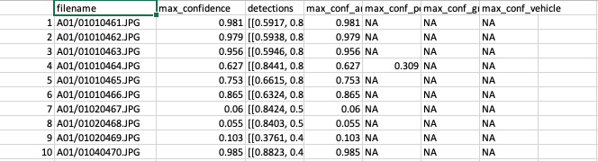
Figure 4.1: Predictions provided by Megadetector.
4.4 Image processing with Timelapse
Timelapse is a software for image processing that can be run in all versions of Microsoft Windows or other operating systems running Windows emulators. Timelapse facilitates image review and annotation of species names or other features of interest (e.g., animals’ sex, behavior, condition, etc.). To run Timelapse, your images must be organized in subfolders (e.g., by study area and camera trap location; Figure 4.2). Timelapse software, video tutorials and a detailed manual with all the software features explained can be downloaded here: http://saul.cpsc.ucalgary.ca/timelapse/pmwiki.php?n=Main.Download2
![Example of image organization in folders and subfolders to load them in Timelapse [@greenberg-timelapse].](input_figures/md/subfolders.png)
Figure 4.2: Example of image organization in folders and subfolders to load them in Timelapse (Greenberg 2020).
Before using Timelapse, you will need to create a data schema (i.e., a template with a .tdb file extension) that identifies the data fields that will be recorded when processing your camera trap data (e.g., species name, sex, behavior, etc.). This step can be accomplished by using the Timelapse Template Editor that is downloaded along with Timelapse. The Template Editor allows you to create the .tdb file that will be read in Timelapse and will adjust the software image processing interface to capture the different data fields you specify in the .tdb file (Greenberg 2020).
Once photos are imported to Timelapse, you can review them using different processing tools provided by the software. The Timelapse manual (Greenberg 2020) and documentation about the software design (Greenberg, Godin, and Whittington 2019) describe in detail the processing tools available in the software, which include features to:
- Magnify images and explore image difference extraction tools (e.g., to identify small animals that are otherwise difficult to spot).
- Select multiple images quickly from small thumbnails and classify them all at once.
- Automate data entry via metadata extraction (time/date, filename, temperature sensed by the camera) and copy annotated information to other images.
- Sort images by date, species or any other annotated feature, to easily review and verify this information.
4.5 Using AI output
To integrate MD output with Timelapse, you will need to have the same folder and subfolder structure (Figure 4.2) that you used when running MD. Using the same folder structure allows Timelapse to match each image with MD output using relative paths associated with each filename.
In Timelapse, you must activate the option for working with image recognition data and import computer vision results stored in the JSON file (Greenberg 2020). You will see bounding boxes that can facilitate image review once the automatic image recognition is activated.
To use AI results to accelerate image review, you can filter MD output categories detected with high confidence levels that are likely correct. To do that, you must provide a confidence range to accept predictions made by computer vision (Figure 4.3). For example, if you choose “Empty” as the detected entity and a high confidence range (e.g, from 0.65 to 1.00), your data set will be filtered to display images predicted as “Empty” by MD and likely to be correct.
![When activating the use of AI detections, users can filter which images are displayed depending on the range of confidence values provided [@greenberg-timelapse].](input_figures/md/confidence_value.png)
Figure 4.3: When activating the use of AI detections, users can filter which images are displayed depending on the range of confidence values provided (Greenberg 2020).
After subsetting images to be displayed depending on their confidence values, you can easily inspect images in the overview mode in Timelapse and select multiple images at a time and assign an “Empty” category to them if the AI output is correct (Figure 4.4). If AI output is not correct, you can edit those classifications.
![Timelapse overview mode where users can perform bulk actions (e.g., selection of multiple images) to accept or edit AI predictions [@greenberg-timelapse].](input_figures/md/overview.png)
Figure 4.4: Timelapse overview mode where users can perform bulk actions (e.g., selection of multiple images) to accept or edit AI predictions (Greenberg 2020).
After, processing images with Timelapse, you can export the data as a CSV File. This file (TimelapseData.csv) will contain all the data entries that you specified in the template (Figure 4.5).
![Output contained in a CSV file exported from Timelapse software [@greenberg-timelapse].](input_figures/md/output.png)
Figure 4.5: Output contained in a CSV file exported from Timelapse software (Greenberg 2020).
4.6 Assessing AI performance
Before exploring model performance with your data, let us recapitulate. MD runs AI models and outputs broad categories of predictions for images (in a JSON file). These AI predictions can be integrated with Timelapse to further process camera trap images (i.e., identifying images with the help of AI output). However, if you have previously classified images (e.g., identified using your software or platform of preference), you can explore MD performance before integrating AI results using Timelapse.
To evaluate MD performance, you will need to 1) classify a subset of your images and export the classification results to a CSV file (containing at minimum, the image filename, camera location and species name), and 2) obtain MD output in CSV format. You can then follow the steps below to evaluate the performance of MD’s AI model. We also discuss how one can select an appropriate confidence threshold for filtering images to accelerate the image review process (e.g., by focusing only on images that likely contain an animal).
4.6.1 Reading in data, introduction to the Purrr package
Below, we demonstrate a step-by-step workflow for how to get MD output into R, join computer and human vision identifications, and estimate model performance metrics for each class. Throughout, we will use the purrr package in R (Henry and Wickham 2020; R Core Team 2021) to repeatedly apply the same function to objects in a list or column in a nested data frame efficiently and without the need for writing loops. Readers unfamiliar with purrr syntax, may want to view one or more of the tutorials, below, or make use of the purrr cheat sheet.
- http://www.rebeccabarter.com/blog/2019-08-19_purrr/
- https://www.r-bloggers.com/2020/05/one-stop-tutorial-on-purrr-package-in-r/
- https://jennybc.github.io/purrr-tutorial/index.html
Once you finish the identification of a subset of your images using your platform of preference, export your classifications as a CSV file and name it as
images_hv.csv. The other CSV file containing the MD results can be named asimages_cv.csv.Create a data folder to store your two CSV files
images_cv.csvandimages_hv.csvthat refer to classifications of computer and human vision, respectively (note, we provide an example of both files with the repository associated with this guide namedimages_cv_jan2020.csvandimages_hv_jan2020.csv).Process the two data files using the R code provided below.
First, we load required libraries and open files.
library(tidyverse) # for data wrangling and visualization, includes dplyr and purrr
library(here) # to allow use of relative paths
Next, we tell R the path (i.e., directory name) that holds our files. We will use the here package (Müller 2017) to tell R that our files live in the “./data/md” directory. You may, alternatively, type in the full path to the file folder or a relative path from the root directory if you are using a project in RStudio.
# Create filefolder's path. This should point to the folder name
# where you stored your CSV files, one with classifications of some of your images
# and the other with MD output
filesfolder <- here("data", "md")
filesfolder
## [1] "/Users/julianavelez/Documents/GitHub/Processing-Camera-Trap-Data-using-AI/data/md"# List your files contained in the filesfolder directory. This code will
# list all your CSV files (i.e., images_cv.csv and images_hv.csv)
files <- dir(filesfolder, pattern = "*.csv")
files## [1] "images_cv_jan2020.csv" "images_hv_jan2020.csv"We then use the map function in the purrr library to read in all of the files and store them in a list object named mycsv. The first argument to map is a list (here, files) which is “piped in” using %>% from the magrittr package (Bache and Wickham 2020). Pipes (%>%) provide a way to execute a sequence of data operations, organized so that the operations can be read from left to right (e.g., “Take the set of files and then read them in using read_csv”). The second argument to map is a function, in this case read_csv, to be applied to the list. The map function iterates over the two files stored in the files object, reads in the data files and then stores them in a new list named mycsv. We use ~ to refer to our function and use .x to refer to the list object that is passed to the function as an additional argument.
# Read both CSV files
mycsv <- files %>%
  map(~read_csv(file.path(filesfolder, .x)))

# Inspect how the data sets look like
mycsv
## [[1]]
## # A tibble: 112,247 × 7
## image_path max_confidence detections max_conf_animal max_conf_person
## <chr> <dbl> <lgl> <dbl> <dbl>
## 1 jan2020/A01/01080001.JPG 0.998 NA NA 0.998
## 2 jan2020/A01/01080002.JPG 0.97 NA NA 0.97
## 3 jan2020/A01/01080003.JPG 0.996 NA NA 0.996
## 4 jan2020/A01/01080004.JPG 0.985 NA 0.202 0.985
## 5 jan2020/A01/01080005.JPG 0.939 NA 0.209 0.939
## 6 jan2020/A01/01080006.JPG 0.996 NA NA 0.996
## 7 jan2020/A01/01080007.JPG 0.999 NA NA 0.999
## 8 jan2020/A01/01080008.JPG 0.997 NA NA 0.997
## 9 jan2020/A01/01080009.JPG 0.914 NA 0.428 0.914
## 10 jan2020/A01/01080010.JPG 0.992 NA NA 0.992
## # … with 112,237 more rows, and 2 more variables: max_conf_group <dbl>,
## # max_conf_vehicle <lgl>
##
## [[2]]
## # A tibble: 103,053 × 5
## filename timestamp image_id common_name sp_num
## <chr> <dttm> <chr> <chr> <dbl>
## 1 N25/03310082.JPG 2020-03-31 14:28:14 902b671f-58b9-4cb… Collared Pecc… 1
## 2 N29/03310288.JPG 2020-03-31 06:49:17 e727dc42-5ebb-46a… Collared Pecc… 1
## 3 A06/06020479.JPG 2020-06-02 08:12:17 db3c3213-5ad9-4bf… Black Agouti 1
## 4 A02/03100387.JPG 2020-03-10 06:58:27 c7e33138-08ac-461… Unknown speci… 1
## 5 A04/04180034.JPG 2020-04-18 05:37:56 52f77e0c-7023-408… Bos Species 1
## 6 A06/03020343.JPG 2020-03-02 12:00:45 94a5b596-1685-40a… Spix's Guan 1
## 7 A06/06190148.JPG 2020-06-19 11:40:33 063c0153-d8fd-46b… White-lipped … 1
## 8 A06/06250315.JPG 2020-06-25 07:08:56 4b6f9c4e-e8bb-4a9… Lowland Tapir 1
## 9 A07/05090248.JPG 2020-05-09 15:05:11 15c4e9f4-7a68-4bd… Domestic Horse 1
## 10 A09/02030454.JPG 2020-02-03 10:34:41 cb56ac06-6520-47c… Bos Species 1
## # … with 103,043 more rows4.6.2 Format computer vision data set
Columns of interest in the the MD data set include:
filename: contains camera location and filename (e.g., A01/01010461.JPG).max_confidence: contains the maximum confidence value found for a detection in an image.max_conf_animal,max_conf_person,max_conf_group,max_conf_vehicle: each of these columns contain a confidence value associated with a prediction by computer vision for the different classes.
We begin by creating a max_conf_blank variable, which we will use to identify blank images. We assign a value of 1 to this variable whenever the observation has missing values for all of the other max_conf variables.
cv_wide <- mycsv %>%
  pluck(1) %>% #extract the computer vision images_cv.csv file
  rename(filename = image_path) %>%
  group_by(filename) %>%
  mutate(max_conf_blank = case_when(sum(is.na(max_conf_animal),
                               is.na(max_conf_person),
                               is.na(max_conf_group),
                               is.na(max_conf_vehicle)) == 4 ~ 1)) %>%
  ungroup()
MD can detect and classify more than one object in an image, and each object will be assigned its own confidence value. We want to keep each of these classifications in a separate row. To do that, we first change the data set from “wide” to “long” format using the pivot_longer function (Wickham and Henry 2018). This function will create two new variables, name and value, that will hold the classification (“Human”, “Animal”, “Vehicle”, “Blank”) and associated confidence values, respectively.
cv_long <- cv_wide %>%
  select(-detections) %>%
  pivot_longer(c("max_conf_animal",
                 "max_conf_person",
                 "max_conf_group",
                 "max_conf_vehicle",
                 "max_conf_blank"))

cv_long
## # A tibble: 561,235 × 4
## filename max_confidence name value
## <chr> <dbl> <chr> <dbl>
## 1 jan2020/A01/01080001.JPG 0.998 max_conf_animal NA
## 2 jan2020/A01/01080001.JPG 0.998 max_conf_person 0.998
## 3 jan2020/A01/01080001.JPG 0.998 max_conf_group NA
## 4 jan2020/A01/01080001.JPG 0.998 max_conf_vehicle NA
## 5 jan2020/A01/01080001.JPG 0.998 max_conf_blank NA
## 6 jan2020/A01/01080002.JPG 0.97 max_conf_animal NA
## 7 jan2020/A01/01080002.JPG 0.97 max_conf_person 0.97
## 8 jan2020/A01/01080002.JPG 0.97 max_conf_group NA
## 9 jan2020/A01/01080002.JPG 0.97 max_conf_vehicle NA
## 10 jan2020/A01/01080002.JPG 0.97 max_conf_blank NA
## # … with 561,225 more rowsNext, we drop all rows where the confidence value is equal to “NA” and rename our classification variable to class. Additionally, we remove images with the “Vehicle” and “Human” classes.
To simplify things, we also change the “Group” label to “Animal”. We do this for 3 reasons: 1) we found that there were very few “Group” classifications in our data set; 2) these predictions were not very accurate; and 3) MD will most often be used to separate blank images from those that have at least one animal present, and thus, the “Group” label is not all that informative.
cv <- cv_long %>%
  filter(is.na(value) != TRUE) %>%
  mutate(name = replace(name, name == "max_conf_blank" , "Blank"),
         name = replace(name, name == "max_conf_animal", "Animal"),
         name = replace(name, name == "max_conf_person", "Human"),
         name = replace(name, name == "max_conf_group", "Animal"),
         name = replace(name, name == "max_conf_vehicle", "Vehicle")) %>%
  rename(class = name) %>%
  filter(!class %in% "Human" & !class %in% "Vehicle")
Changing the “Group” label to “Animal” results in some images having multiple predictions of “Animal” for the same image. In these cases, we use the top_n function to select the record with the highest confidence value (Wickham et al. 2019).
cv <- cv %>%
        group_by(filename, class) %>%
        top_n(1, value) %>% # keep highest value of same class
        group_by(filename, class) %>%
        distinct(filename, class, value, .keep_all = TRUE) # for filenames with the same confidence value, keep a single record
Comparing output from human and computer vision also requires that the classification variables have the same levels attribute. We first create a vector, all_levels, containing the names of the classes. Then, we use the factor function (R Core Team 2021) to convert common names into factor classes and assign the levels to the class column.
# Create a vector with levels of predicted categories
all_levels <- c("Animal", "Blank")

# Assign the levels attribute to the class column
cv$class <- factor(as.character(cv$class, levels = all_levels))
Lastly, we add a variable that will indicate if there are multiple detections within the same image.
4.6.3 Format human vision data set
The human vision data set (ìmages_hv_jan2020.csv) was previously cleaned to remove duplicated records and to summarize multiple rows that reference animals of the same species identified in the same image (see Chapter 3) for details about these steps).
We begin by inspecting all the species names contained in the human vision data set using the unique function (R Core Team 2021). We will eventually need to create a variable that can be compared to MD output (i.e., broad classes identifying “Blank” and “Animal”).
hv_sp <- mycsv %>%
  pluck(2) # select human vision data frame

# check all species present in the data set
unique(hv_sp$common_name) %>% sort()
## [1] "Alouatta Species" "Amazonian Motmot"
## [3] "Ants" "Bird"
## [5] "Black Agouti" "Blank"
## [7] "Bos Species" "Bush Dog"
## [9] "Caprimulgidae Family" "Capybara"
## [11] "Cervidae Family" "Collared Peccary"
## [13] "Common Green Iguana" "Crab-eating Fox"
## [15] "Crestless Curassow" "Dasypus Species"
## [17] "Domestic Dog" "Domestic Horse"
## [19] "Fasciated Tiger-heron" "Giant Anteater"
## [21] "Giant Armadillo" "Giant Otter"
## [23] "Insect" "Jaguar"
## [25] "Jaguarundi" "Lizards and Snakes"
## [27] "Lowland Tapir" "Mammal"
## [29] "Margarita Island Capuchin" "Margay"
## [31] "Northern Amazon Red Squirrel" "Ocelot"
## [33] "Ornate Tití Monkey" "Pecari Species"
## [35] "Possum Family" "Puma"
## [37] "Red Brocket" "Rodent"
## [39] "Saimiri Species" "South American Coati"
## [41] "Southern Tamandua" "Spix's Guan"
## [43] "Spotted Paca" "Tayra"
## [45] "Turkey Vulture" "Turtle Order"
## [47] "Unknown species" "Weasel Family"
## [49] "White-lipped Peccary" "White-tailed Deer"MD output represents filenames as “deployment/camera_location/image_filename”, based on folder structure. We add the deployment name to the filename variable in human vision output so that it matches the format of the MD data set. These steps will allow us to later join our human and computer vision data sets using the common variable, filename.
We use the case_when function (Wickham et al. 2019) to implement multiple conditional statements to create a variable, class_hv, containing the classes found in MD output. We select the columns of interest, including a newly created variable (multiple_det) that will keep track of images that have two or more species present in the same image, each recorded in a different row. For the multiple detections, we keep a single row using the distinct function (Wickham et al. 2019).
We also assign a levels attribute to the class variable in human vision so that it is comparable to the class variable in the computer vision data set.
hv <- hv_sp %>%
  group_by(filename, timestamp) %>%
  mutate(multiple_det = n() > 1) %>% # create multiple detections column (TRUE/FALSE).
  mutate(class = case_when(common_name == "Blank" ~ common_name,
                           TRUE ~ "Animal")) %>%
  select(filename, timestamp, class, multiple_det)

hv <- hv %>%
  group_by(filename, class) %>%
  distinct(filename, class, .keep_all = TRUE) %>%
  ungroup()

# Assign the levels attribute to the class column
hv$class <- factor(as.character(hv$class), levels = all_levels)
4.6.4 Merging computer and human vision data sets
Now that we have the same format for both human and computer vision data sets, we can use various “joins” (Wickham et al. 2019) to merge the two data sets together so that we can evaluate the accuracy of MD. First, however, we will eliminate any images that were not processed by both humans and AI.
# Determine which images have been viewed by both methods
ind1 <- cv$filename %in% hv$filename # in both
ind2 <- hv$filename %in% cv$filename # in both

cv <- cv[ind1,] # eliminate images not processed by hv
hv <- hv[ind2,] # eliminate images not processed by cv

# Number of photos eliminated
sum(ind1 != TRUE) # in cv but not in hv
## [1] 5397## [1] 1168Now, we can use:
- an
inner_joinwithfilenameandclassto determine images that have correct predictions (i.e., images with the same class assigned by computer and human vision) - an
anti_joinwithfilenameandclassto determine which records in the human vision data set have incorrect predictions from computer vision. - an
anti_joinwithfilenameandclassto determine which records in the computer vision data set have incorrect predictions.
We assume the classifications from human vision to be correct and distinguish them from MD predictions. The MD predictions will be correct if they match a class assigned by human vision for a particular record and incorrect if the classes assigned by the two visions differ.
# correct predictions
matched <- cv %>%
  inner_join(y = hv, by = c("filename", "class"), suffix = c("_cv", "_hv")) %>%
  mutate(class_hv = class) %>%
  rename(class_cv = class) %>%
  select(filename, value, class_cv, class_hv, multiple_det_cv, multiple_det_hv)

# incorrect predictions in hv set
hv_only <- hv %>%
  anti_join(y = cv, by = c("filename", "class"), suffix = c("_hv", "_cv")) %>%
  rename(class_hv = class) %>%
  rename(multiple_det_hv = multiple_det)

# incorrect predictions in cv set
cv_only<- cv %>%
  anti_join(y = hv, by = c("filename", "class"), suffix = c("_cv", "_hv")) %>%
  rename(class_cv = class)
We then use left_join to merge the predictions from the cv_only (computer vision) data set onto the records from the hv_only (human vision) data set.
hv_mismatch <- hv_only %>%
  left_join(cv_only, by = "filename") %>%
  rename(multiple_det_cv = multiple_det) %>%
  select(filename, value, class_cv, class_hv, multiple_det_cv, multiple_det_hv)
We then check for any computer vision records that are not yet accounted for in our data sets containing records with correct or incorrect predictions, i.e., matched and hv_mismatch, respectively.
cv_others <- cv_only[cv_only$filename %in% matched$filename != TRUE,]
cv_others <- cv_only[cv_only$filename %in% hv_mismatch$filename != TRUE,]

table(cv_others$multiple_det)
## < table of extent 0 >## < table of extent 0 >Then, we select only the variables we need, combine the matched and mismatched data sets, and again make sure that the classifications have the same factor levels attribute.
matched <- matched %>%
  select(filename, value, class_cv, class_hv)
hv_mismatch <- hv_mismatch %>%
  select(filename, value, class_cv, class_hv)

both_visions <- rbind(matched, hv_mismatch)
both_visions$class_cv <- factor(as.character(both_visions$class_cv), levels = all_levels)
both_visions$class_hv <- factor(as.character(both_visions$class_hv), levels = all_levels)
4.6.5 Confusion matrix and performance measures
Finally, we can proceed with estimating a confusion matrix and various AI performance measures using the confusionMatrix function from the caret package (Kuhn 2021) and specifying a 0.65 confidence threshold to accept MD predictions. We can then plot the confusion matrix using ggplot2 (Wickham et al. 2018). The confusionMatrix function requires a data argument for predicted classes and a reference for true classifications, both as factor classes and with the same factor levels. We specify mode = "prec_recall" when calling the confusionMatrix function (Kuhn 2021) to generate estimates of precision and recall.
library(caret) # to inspect model performance
library(ggplot2)

# Estimate confusion matrix
both_visions_0.65 <- both_visions
both_visions_0.65$class_cv[both_visions_0.65$value < 0.65] <- "Blank"
cm_md_0.65 <- confusionMatrix(data = both_visions_0.65$class_cv,
                      reference = both_visions_0.65$class_hv,
                      mode = "prec_recall")

# Plot confusion matrix
plot_cm_md_0.65 <- cm_md_0.65 %>%
  pluck("table") %>%
  as.data.frame() %>%
  rename(Frequency = Freq) %>%
  ggplot(aes(y=Prediction, x=Reference, fill=Frequency)) +
  geom_raster() +
  scale_fill_gradient(low = "#D6EAF8",high = "#2E86C1") +
  theme(axis.text.x = element_text(angle = 90)) +
  geom_text(aes(label = Frequency), size = 3) #set size to 3

plot_cm_md_0.65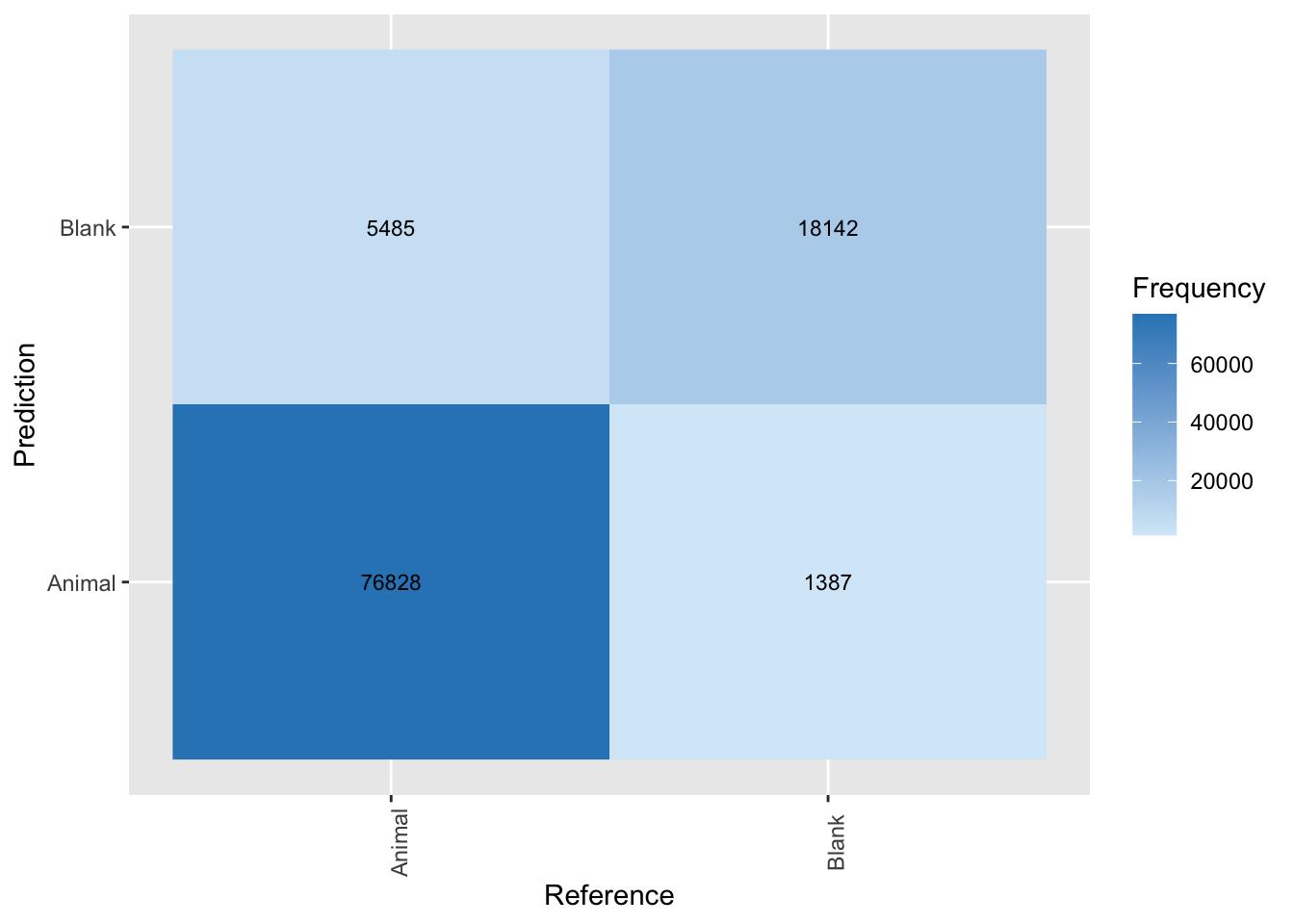
Figure 4.6: Confusion matrix applied to classifications from MegaDetector using a confidence threshold of 0.65.
Now we can use the confusion matrix to estimate metrics of model performance including accuracy, precision, recall and F1 score (See Chapter 1 for metrics description).
## [1] 0.93classes_metrics_md_0.65 <- cm_md_0.65 %>%
pluck("byClass") %>%
t() %>%
as.data.frame() %>%
select(Precision, Recall, F1) %>%
mutate(across(where(is.numeric), ~round(., 2)))
classes_metrics_md_0.65 <- classes_metrics_md_0.65 %>%
mutate(Class = "Animal", .before = Precision)We see that the model is really good at picking up animals, with a precision of 98% at a 93% recall. Thus, we expect that 93% of the animals present in our images will be picked up by MD. Further, only 2% of the images flagged as having an animal will not. We can also inspect model performance for a range of confidence thresholds as we demonstrate in the next section.
4.6.6 Confidence thresholds
Lets begin by looking at the confidence values associated with each MD classification using the geom_bar function (Wickham et al. 2018). Before plotting, we filter the both_visions data frame to remove blanks as they do not have associated confidence values.
# Plot confidence values
both_visions %>%
  filter(class_cv != "Blank") %>%
  ggplot(aes(value, group = class_cv, colour = class_cv)) +
  geom_bar() +
  facet_wrap(~class_cv, scales = "free") +
  labs(y = "Empirical distribution", x = "Confidence values") +
  scale_color_viridis_d()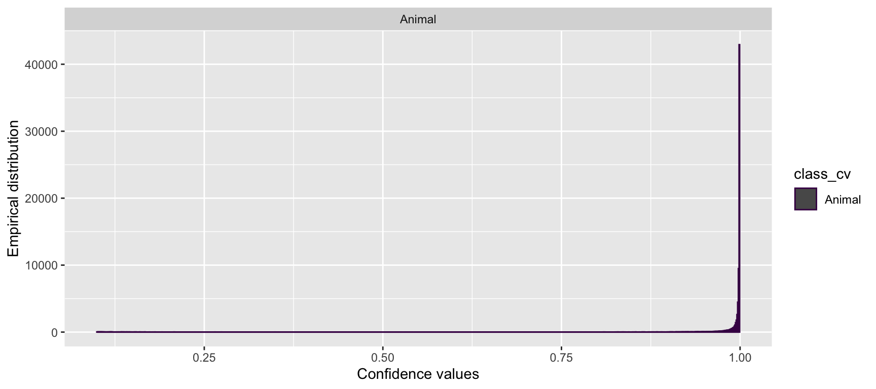
Figure 4.7: Distribution of confidence values for animals predicted by MegaDetector.
We see that the distribution of confidence values for “Animal” classifications is left skewed with most records having high confidence values suggesting that the AI prediction is presumed to be correct most of the time.
To inspect how precision and recall change when different confidence thresholds are established for assigning a class predicted by computer vision, we define a function that will calculate these metrics for a user-defined confidence threshold. This function will assign a “Blank” label whenever the confidence for a computer vision prediction is below a particular confidence threshold. Higher thresholds should reduce the number of false positives but at the expense of more false negatives. We then estimate the same performance metrics for the specified confidence threshold. By repeating this process for several different thresholds, users can evaluate how precision and recall change with the confidence threshold and choose a threshold that balances these two performance metrics.
threshold_for_metrics <- function(conf_threshold = 0.7) {
  tmp <- both_visions
  tmp$class_cv[tmp$value < conf_threshold] <- "Blank"

  cm <- confusionMatrix(data = tmp$class_cv,
                        reference = tmp$class_hv,
                        mode = "prec_recall")

  classes_metrics <- cm %>% # get confusion matrix
    pluck("byClass") %>% # get metrics by class
    t() %>%
    as.data.frame() %>%
    select(Precision, Recall, F1) %>%
    mutate(conf_threshold = conf_threshold)

  return(classes_metrics) # return a data frame with metrics for every class
}
Let’s estimate model performance metrics for confidence values ranging from 0.1 to 0.99 using the map_df function (Henry and Wickham 2020) . The map_df function (Henry and Wickham 2020) returns a data frame object. Once we get a data frame of model performance metrics for a range of confidence values, we can plot the results using the ggplot2 package (Wickham et al. 2018).
conf_vector = seq(0.1, 0.99, length=100)

metrics_all_confs <- map_df(conf_vector, threshold_for_metrics)
prec_rec_md <- metrics_all_confs %>%
rename(`Confidence threshold` = conf_threshold) %>%
ggplot(aes(x = Recall, y = Precision)) +
geom_point(aes(size = `Confidence threshold`, color = "#440154FF")) +
scale_size(range = c(0.1,3)) +
labs(x = "Recall", y = "Precision")+
geom_line(color = "#440154FF") +
scale_color_manual(values = "#440154FF", name = "Class", labels = "Animal") +
xlim(0, 1) + ylim(0, 1)
prec_rec_md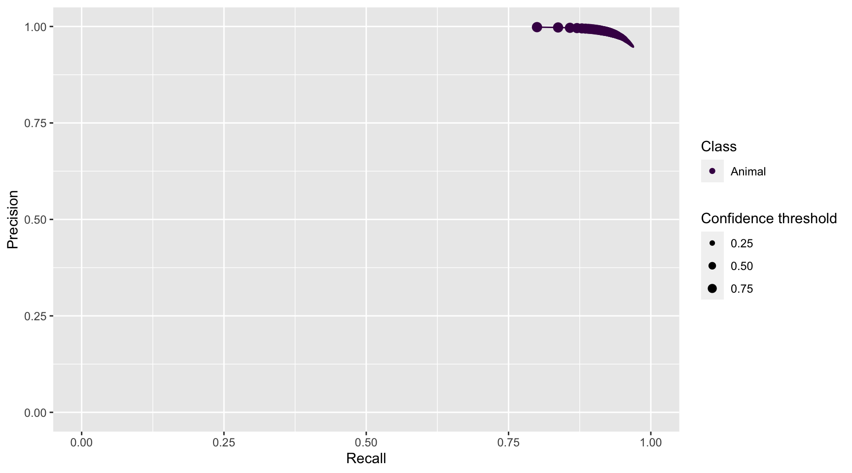
Figure 4.8: Precision and recall for different confidence thresholds for the animal class predicted by MegaDetector.
We see that as we increase the confidence threshold, precision increases and recall decreases for the “Animal” class (Figure 4.8). Ideally, we would like to choose a confidence threshold that maximizes both precision and recall, though the latter is likely to be more important in most cases. Remember that precision tells us the probability that the class is truly present when AI identifies the class as being present in an image (Chapter 1). If AI suffers from low precision, then we may have to manually review photos that AI tags as having a class present in order to remove false positives. Recall, on the other hand, tells us how likely AI is to find a class in the image when it is truly present. If AI suffers from low recall, then it will miss many photos containing a class that is truly present. To remedy this problem, we would need to review images where AI says the class is absent in order to reduce false negatives.
Let’s say that we were willing to miss only 3% of the animals present. In this case, we could pick the confidence threshold that maximizes precision under the constraint that recall does not fall below 97%.
conf_meets <- metrics_all_confs %>%
  mutate(across(where(is.numeric), ~round(., 2))) %>%
filter(Recall >= 0.97)| Precision | Recall | F1 | conf_threshold |
|---|---|---|---|
| 0.95 | 0.97 | 0.96 | 0.1 |
We see that we can obtain a precision to 95% (while keeping recall = 97%) by using a confidence threshold of 0.1. Thus, if we integrate MD output with Timelapse, filtering using a confidence threshold of 0.1, we expect to capture 97% of Animals that are truly present and 95% of the flagged images should actually include one or more animals.
Let’s examine the confusion matrix using this threshold.
threshold <- conf_meets[which.max(conf_meets$Precision), 4]

conf_red <- both_visions
conf_red$class_cv[conf_red$value < threshold] <- "Blank"


cm_md_th <- confusionMatrix(data = conf_red$class_cv,
                        reference = conf_red$class_hv,
                        mode = "prec_recall")

plot_cm_md_th <- cm_md_th %>%
        pluck("table") %>%
        as.data.frame() %>%
        rename(Frequency = Freq) %>%
        ggplot(aes(y=Prediction, x=Reference, fill=Frequency)) +
  geom_raster() +
  scale_fill_gradient(low = "#D6EAF8",high = "#2E86C1") +
  theme(axis.text.x = element_text(angle = 90)) +
geom_text(aes(label = Frequency), size = 3)library(patchwork)
plot_cm_md_0.65 <- plot_cm_md_0.65 + theme(legend.position = "None")
plot_cm_md_th <- plot_cm_md_th + theme(legend.position = "None")
(plots_cms_md <- plot_cm_md_0.65 +
plot_cm_md_th +
plot_annotation(tag_levels = 'A'))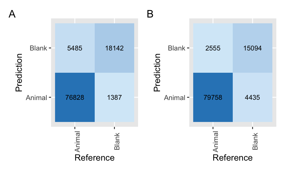
Figure 4.9: Confusion matrices applied to classifications from MegaDetector using a confidence threshold of 0.65 (A) and 0.1 (B).
Comparing the confusion matrix with our original (using a 0.65 confidence threshold; Figure 4.9), we see that we have decreased the false negatives using a confidence threshold of 0.1 (i.e., cases where MD suggests a blank image but an animal is present; last row, first column) but increased the number of false positives (i.e., cases where MD suggests an animal is present, but the image is blank; first row, second column).
4.7 Conclusions
We have seen how to use MD and how to integrate its output with Timelapse for using AI while processing camera trap data. Additionally, we illustrated how to evaluate MD performance by comparing true classifications with computer predictions. We found that MD has a high performance to detect animals in images. Thus, the human labor required to review photos can be reliably focused on images with the “Animal” class predictions.
We also showed how users can explore MD performance by comparing confusion matrices estimated using different confidence thresholds. This comparison will be useful to understand the trade-off between precision and recall, and help users choose a confidence threshold that maximizes these metrics using their particular data sets.
References
Bache, Stefan Milton, and Hadley Wickham. 2020. Magrittr: A Forward-Pipe Operator for R. https://CRAN.R-project.org/package=magrittr.
Beery, Sara, Dan Morris, and Siyu Yang. 2019. “Efficient Pipeline for Camera Trap Image Review.” arXiv Preprint arXiv:1907.06772.
Greenberg, Saul. 2020. “Timelapse 2.0 User Guide.” Computer Program. Greenberg Consulting Inc. / University of Calgary.
Greenberg, Saul, Theresa Godin, and Jesse Whittington. 2019. “Design Patterns for Wildlife-Related Camera Trap Image Analysis.” Journal Article. Ecology and Evolution 9 (24): 13706–30. https://doi.org/10.1002/ece3.5767.
Henry, Lionel, and Hadley Wickham. 2020. Purrr: Functional Programming Tools. https://CRAN.R-project.org/package=purrr.
Kuhn, Max. 2021. Caret: Classification and Regression Training. https://CRAN.R-project.org/package=caret.
Müller, Kirill. 2017. Here: A Simpler Way to Find Your Files. https://CRAN.R-project.org/package=here.
R Core Team. 2021. R: A Language and Environment for Statistical Computing. Vienna, Austria: R Foundation for Statistical Computing. https://www.R-project.org/.
Wickham, Hadley, Winston Chang, Lionel Henry, Thomas Lin Pedersen, Kohske Takahashi, Claus Wilke, and Kara Woo. 2018. Ggplot2: Create Elegant Data Visualisations Using the Grammar of Graphics. https://CRAN.R-project.org/package=ggplot2.
Wickham, Hadley, Romain François, Lionel Henry, and Kirill Müller. 2019. Dplyr: A Grammar of Data Manipulation. https://CRAN.R-project.org/package=dplyr.
Wickham, Hadley, and Lionel Henry. 2018. Tidyr: Easily Tidy Data with ’Spread()’ and ’Gather()’ Functions. https://CRAN.R-project.org/package=tidyr.